About pandapipes

pandapipes is an easy to use network calculation program aimed at automation of analysis of district heating and gas systems. It utilizes the data analysis library pandas and is also closely related to the power systems calculation program pandapower.

pandapipes and pandapower can be used in combination to analyze multi energy networks. An environment able to couple both tools is pandapowerpro.

Why another tool?

Motivation

Multi-Energy networks and the utilization of synergies between energy sectors are an important research topic today. To simulate these networks, it is crucial to not only include coupling points between the sectors in the analysis, but also to know the network state of sectors of interest. pandapipes was developed to provide a tool capable of calculating state variables of multi-energy networks. To do so, it can be used in combination with the open source software pandapower. If only gas or district heating networks are of interest, pandapipes can also be used as a stand-alone application.

In this sense, pandapipes closes two gaps: There are not many tools available which focus on multi-energy grid modeling. In addition, most software for calculating fluid networks is only commercially available. The following table summarizes some properties of commercial and open source tools, respectively.

	Fluid Models	Automation	Customization
Commercial Tools (e.g. Stanet, Sincal, NEPLAN)	Thoroughly validated and easy to parametrize models of pipes, pumps, valves etc. Typically, multi-energy networks are not considered.	Graphical User Interface (GUI) applications that are difficult to automate.	Restricted possibilities for customization due to proprietary code base.
Open Source Tools (e.g. Modelica, TransientEE)	Models that require parametrization by the user with expert knowledge.	Console or GUI applications that might be automized.	Open Source code base that can be freely modified and customized.
pandapipes	Thoroughly validated and easy to parametrize fluid models of pipes, pumps, valves etc. with the focus on multi-energy grids.	Console application that is designed for automated evaluations.	Open source code base that can be freely modified and customized.

This is of course a very broad classification of tools that is only supposed to illustrate the focus of pandapipes without considering the diverse landscape of existing tools.

Scope

pandapipes is aimed at static analysis of balanced fluid systems. This allows analysis of:

• Static or quasi-static analyses of pressure and velocity distributions in fluid networks using incompressible or compressible media. Gas composition is assumed fix.
• Static or quasi-static analyses of temperature distributions in fluid networks. At present, this kind of analysis is only possible for incompressible media.

Fluid System Modeling

Tabular Data Structure

pandapipes is based on a tabular data structure, where every element type is represented by a table that holds all parameters for a specific element and a result table which contains the element specific results of the different analysis methods. The tabular data structure is based on the Python library pandas. It allows storing variables of any data type, so that parameters can be stored together with status variables and meta-data, such as names or descriptions. The tables can be easily expanded and customized by adding new columns without influencing the pandapipes functionality. All inherent pandas methods can be used to efficiently read, write and analyze the network and results data.

Standard Type Libraries

pandapipes includes a standard type library that allows the creation of pipes and pumps using predefined basic standard type parameters. The user can either define individual standard types or use the predefined pandapipes basic standard types for convenient definition of networks.

Fluid Property Library

pandapipes includes a fluid property library that allows the creation of fluid properties using predefined data. The user can either define individual properties or use the predefined data.

Fluid System Analysis

pandapipes supports the following fluid systems analysis functions:

• Pipe Flow

Pipe Flow

The pandapipes pipe flow solver is based on the Newton-Raphson method.
Learn more
To initialize the solution vector for the pipe flow calculation pandapipes offers two different methods:

• flat start
• solution vector of a previous calculation

Tests and Validation

So far pandapipes has been successfully tested with pytest. To ensure the correctness of the functionalities in pandapipes, various test networks were created, in which different factors were varied:

• medium: gas and water
• topology
• pressure at external grids
• number of external grids
• friction model
• length, diameter and roughness of a pipe
• volume flow
• number and height values of nodes
• direction of pipe link between nodes, for checking the correct flow velocity calculation
• combinations of sources, sinks, pumps, valves and external grids
• heat network calculation (only with OpenModelica)

The test networks were created in STANET and OpenModelica and transformed into a pandapipes network using the respective converter to perform the tests in PyCharm. A total of 83 tests were created using both programs. 22 water and 21 gas networks with STANET and 32 water and 8 heating networks with OpenModelica. How to call up the individual example networks is described in the Networks chapter of the documentation. The structures of all test networks are listed below:

The pandapipes test networks.

Legend of the network components.

STANET Tests

The STANET test nets were saved in CSV format so that a conversion into a json file can take place. A test is considered passed, if certain error tolerances are met. The relative error $\mathrm{p_diff}$ during the calculation of the pressures mostly has a value less than 0.002. In two cases the limit has to be increased, once to 0.01 and the second time to 0.03.

$\mathrm{p_diff}=\left|\right(\mathrm{p_stanet}-\mathrm{p_pandapipes})/\mathrm{p_stanet}|$

Furthermore, the absolute error in the calculation of the flow velocities $\mathrm{v_diff,abs}$ is always less than 0.03.

$\mathrm{v_diff,abs}=|\mathrm{v_stanet}-\mathrm{v_pandapipes}|$

OpenModelica Tests

Using the mo- and a mat-file containing the simulation results, the OpenModelica net will be converted into a pandapipes network. OpenModelica uses the Navier-Stokes equations to calculate pressure loss and flow velocities. Whereas pandapipes uses an approach similar to STANET. Consequently, the tolerances for errors for passing a test should be increased. For the relative error $\mathrm{p_diff}$ with respect to pressure, a limit of 0.01 is usually sufficient. In 3 cases the limit should be increased to 0.02 and in 2 cases to 0.06 and 0.4 respectively. Presumably, the deviations are caused by the complexity of the networks, in which pumps and valves are usually found. However, it is not generally due to the use of pumps and valves, since test networks with pumps and valves that maintain a fault tolerance of 0.01 also exist. In addition, the limit for the relative pressure deviation for heating networks lies in a range between 0.01 and 0.05.

$\mathrm{p_diff}=\left|\right(\mathrm{p_modelica}-\mathrm{p_pandapipes})/\mathrm{p_modelica}|$

Furthermore, the absolute error for the flow velocities $\mathrm{v_diff,abs}$ is always below 0.05.

$\mathrm{v_diff,abs}=|\mathrm{v_modelica}-\mathrm{v_pandapipes}|$

For the thermal network calculation, the upper tolerance value for the relative error of the mean temperatures $\mathrm{T_diff,mean}$ is in a range from 0.004 to 0.04.

$\mathrm{T_diff,mean}=\left|\right(\mathrm{T_{mean,modelica}}-\mathrm{T_{mean,pandapipes}})/\mathrm{T_{mean,modelica}}|$

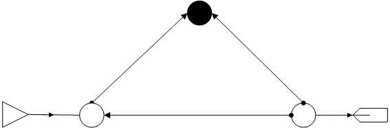
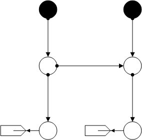
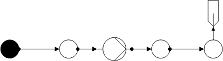
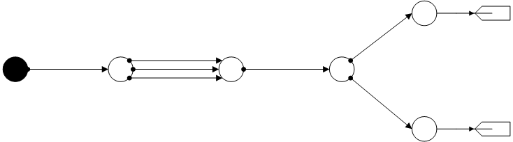
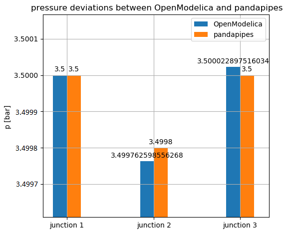
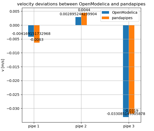
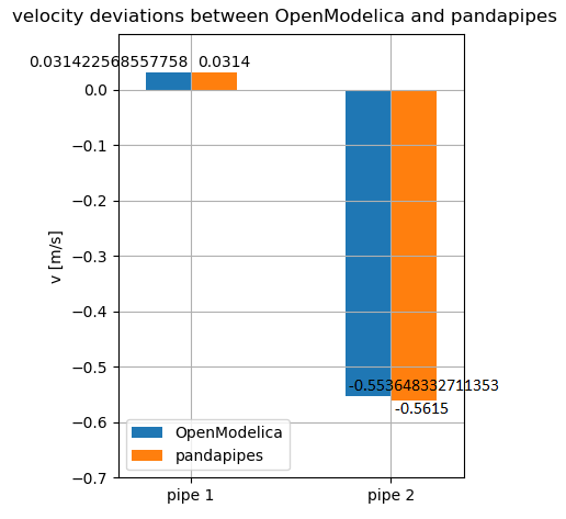
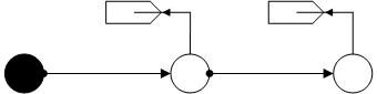
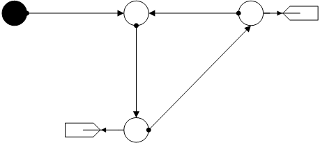
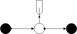
In the following, the deviations of pressures and flow velocities from the OpenModelica and pandapipes calculations are graphically displayed for three different networks. The first net is the Delta net calculated with Prandtl-Colebrook where $\mathrm{p_diff}$ is less than 0.01:

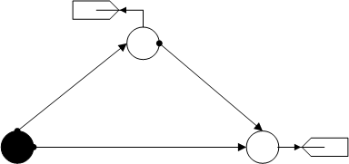
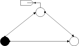
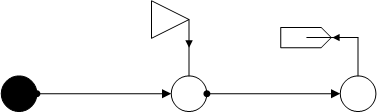
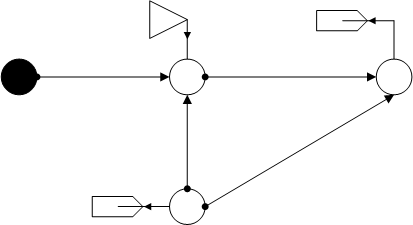
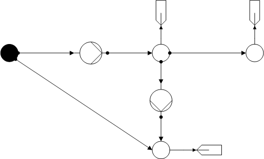
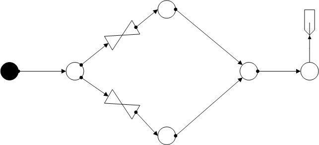
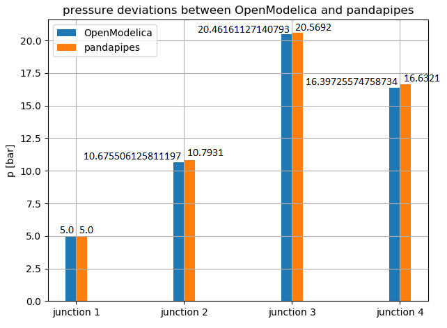
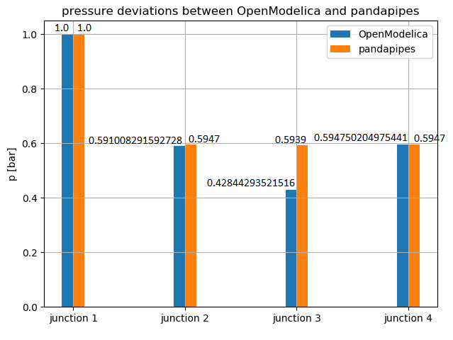
For the Pumps net using Swamee-Jain for calculation, $\mathrm{p_diff}$ is below 0.02 and has the below deviations in the junctions and the pipes:

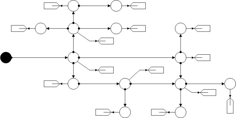
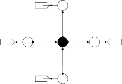
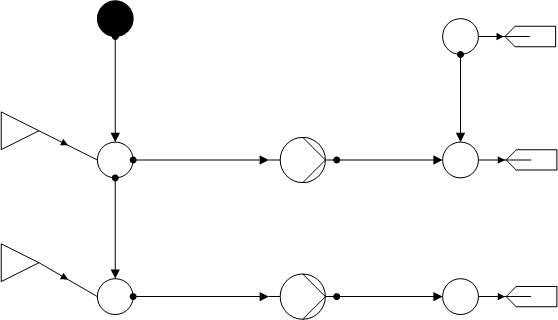
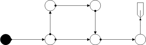
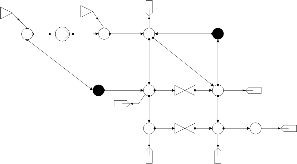
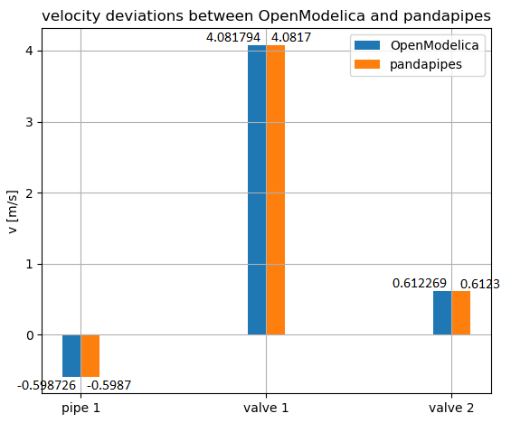
At last the deviations for a network with valves are shown. Here, a limit of 0.4 must be set for the relative error with respect to pressure to pass the test. The Valves network was calculated with Prandtl-Colebrook:

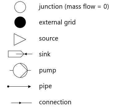
In order to create your own nets in OpenModelica and to perform a comparison with pandapipes, the elements that serve as equivalents for the components in pandapipes are listed hereafter:

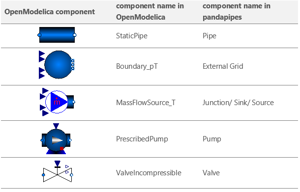
In the case of heat network calculation, the DynamicPipe must be used instead of the StaticPipe:

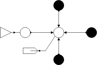
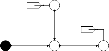
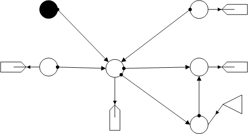
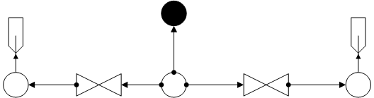
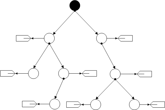
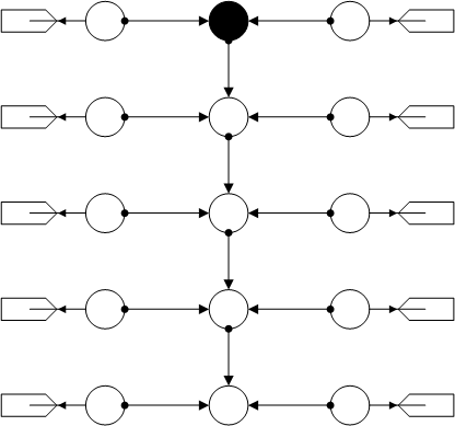
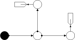
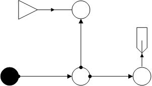
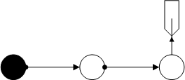
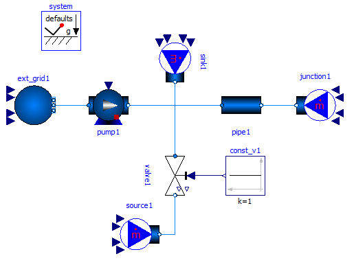
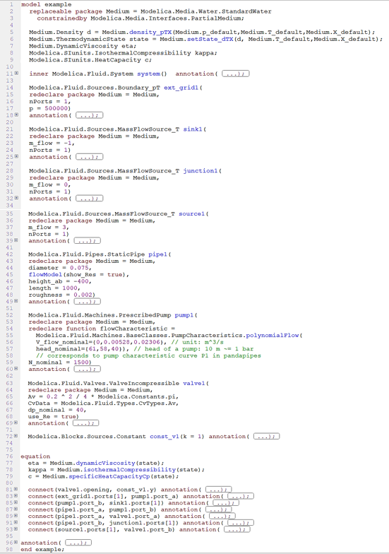
Example

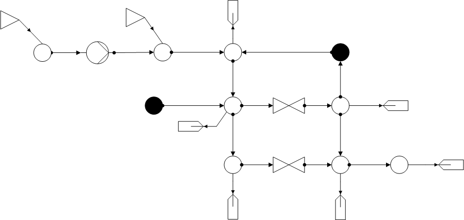
In the following section an example is presented in which all the above mentioned components except the DynamicPipe appear. The components have the below parameters:

Component	Parameter
External Grid (ext_grid1)	p = 5 bar
Sink (sink1)	m_flow = -1 kg/s
Source (source1)	m_flow = 3 kg/s
Junction (junction1)	m_flow = 0 kg/s
Pipe (pipe1)	length = 1km diameter = 0.075 m roughness = 2 mm height_ab = -400 m
Valve (valve1)	A ~= 0,031416 m^2
Constant (const_v1)	k = 1 (valve opened)
Pump (pump1)	pump characteristic curve P1 in pandapipes

The medium is water with a temperature of 293.15 K, where the ambient temperature has the same value. The fluid properties can be called using special methods in OpenModelica, for this purpose the source code must be considered.

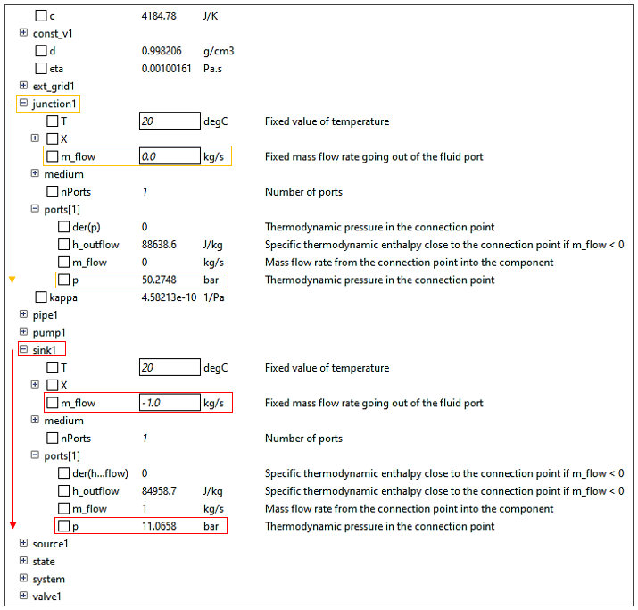
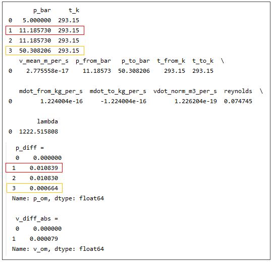
The results of the calculations are shown in the following. The results for junction1 and sink1 are highlighted in color. Also the deviations of the comparison are listed further down.

Results of OpenModelica calculations with Prandtl-Colebrook.

Results of the pandapipes calculations with Prandtl-Colebrook and the results of the comparison with the OpenModelica simulation.

Citing pandapipes

If you use pandapipes in your work, we kindly ask you to cite the pandapipes reference paper

License

pandapipes is published under the following 3-clause BSD license:

Copyright (c) 2020-2021 by Fraunhofer Institute for Energy Economics and Energy System Technology (IEE) Kassel and individual contributors (see AUTHORS file for details). All rights reserved. Redistribution and use in source and binary forms, with or without modification, are permitted provided that the following conditions are met:

1. Redistributions of source code must retain the above copyright notice, this list of conditions and the following disclaimer.

2. Redistributions in binary form must reproduce the above copyright notice, this list of conditions and the following disclaimer in the documentation and/or other materials provided with the distribution.

3. Neither the name of the copyright holder nor the names of its contributors may be used to endorse or promote products derived from this software without specific prior written permission.

THIS SOFTWARE IS PROVIDED BY THE COPYRIGHT HOLDERS AND CONTRIBUTORS “AS IS” AND ANY EXPRESS OR IMPLIED WARRANTIES, INCLUDING, BUT NOT LIMITED TO, THE IMPLIED WARRANTIES OF MERCHANTABILITY AND FITNESS FOR A PARTICULAR PURPOSE ARE DISCLAIMED. IN NO EVENT SHALL THE COPYRIGHT HOLDER OR CONTRIBUTORS BE LIABLE FOR ANY DIRECT, INDIRECT, INCIDENTAL, SPECIAL, EXEMPLARY, OR CONSEQUENTIAL DAMAGES (INCLUDING, BUT NOT LIMITED TO, PROCUREMENT OF SUBSTITUTE GOODS OR SERVICES; LOSS OF USE, DATA, OR PROFITS; OR BUSINESS INTERRUPTION) HOWEVER CAUSED AND ON ANY THEORY OF LIABILITY, WHETHER IN CONTRACT, STRICT LIABILITY, OR TORT (INCLUDING NEGLIGENCE OR OTHERWISE) ARISING IN ANY WAY OUT OF THE USE OF THIS SOFTWARE, EVEN IF ADVISED OF THE POSSIBILITY OF SUCH DAMAGE.